Dimensionality reduction
Timothy Keyes
2024-08-25
Source:vignettes/dimensionality-reduction.Rmd
dimensionality-reduction.RmdA useful tool for visualizing the phenotypic relationships between single cells and clusters of cells is dimensionality reduction, a form of unsupervised machine learning used to represent high-dimensional datasets in a smaller number of dimensions.
tidytof includes several dimensionality reduction
algorithms commonly used by biologists: Principal component analysis
(PCA), t-distributed stochastic neighbor embedding (tSNE), and uniform
manifold approximation and projection (UMAP). To apply these to a
dataset, use tof_reduce_dimensions().
Dimensionality reduction with
tof_reduce_dimensions().
Here is an example call to tof_reduce_dimensions() in
which we use tSNE to visualize data in tidytof’s built-in
phenograph_data dataset.
data(phenograph_data)

# perform the dimensionality reduction
phenograph_tsne <-
    phenograph_data |>
    tof_preprocess() |>
    tof_reduce_dimensions(method = "tsne")
#> Loading required namespace: Rtsne

# select only the tsne embedding columns
phenograph_tsne |>
    select(contains("tsne")) |>
    head()
#> # A tibble: 6 × 2
#>   .tsne1 .tsne2
#>    <dbl>  <dbl>
#> 1   1.74  17.0
#> 2  10.4    7.60
#> 3  30.4   19.8
#> 4  15.2   14.6
#> 5   3.99  19.0
#> 6  21.3   12.4
By default, tof_reduce_dimensions will add
reduced-dimension feature embeddings to the input tof_tbl
and return the augmented tof_tbl (that is, a
tof_tbl with new columns for each embedding dimension) as
its result. To return only the features embeddings themselves, set
augment to FALSE (as in
tof_cluster).
phenograph_data |>
    tof_preprocess() |>
    tof_reduce_dimensions(method = "tsne", augment = FALSE)
#> # A tibble: 3,000 × 2
#>    .tsne1 .tsne2
#>     <dbl>  <dbl>
#>  1  18.7  -1.60
#>  2   9.55  3.71
#>  3  11.3  27.9
#>  4  14.8  13.4
#>  5  20.9   0.568
#>  6  23.3  14.5
#>  7  19.0   6.40
#>  8  27.1  14.7
#>  9  20.1  12.6
#> 10  12.7  -1.41
#> # ℹ 2,990 more rows
Changing the method argument results in different
low-dimensional embeddings:
phenograph_data |>
    tof_reduce_dimensions(method = "umap", augment = FALSE)
#> # A tibble: 3,000 × 2
#>    .umap1 .umap2
#>     <dbl>  <dbl>
#>  1 -5.17  -5.17
#>  2 -5.76  -4.26
#>  3 -7.72   0.819
#>  4 -6.54   0.271
#>  5 -4.95  -4.90
#>  6 -0.380  3.52
#>  7 -4.76  -4.44
#>  8 -7.57   1.40
#>  9 -6.43  -0.919
#> 10 -6.92  -6.41
#> # ℹ 2,990 more rows

phenograph_data |>
    tof_reduce_dimensions(method = "pca", augment = FALSE)
#> # A tibble: 3,000 × 5
#>       .pc1     .pc2   .pc3    .pc4   .pc5
#>      <dbl>    <dbl>  <dbl>   <dbl>  <dbl>
#>  1 -2.77    1.23    -0.868  0.978   3.49
#>  2 -0.969  -1.02    -0.787  1.22    0.329
#>  3 -2.36    2.54    -1.95  -0.882  -1.30
#>  4 -3.68   -0.00565  0.962  0.410   0.788
#>  5 -4.03    2.07    -0.829  1.59    5.39
#>  6 -2.59   -0.108    1.32  -1.41   -1.24
#>  7 -1.55   -0.651   -0.233  1.08    0.129
#>  8 -1.18   -0.446    0.134 -0.771  -0.932
#>  9 -2.00   -0.485    0.593 -0.0416 -0.658
#> 10 -0.0356 -0.924   -0.692  1.45    0.270
#> # ℹ 2,990 more rows
Method specifications for tof_reduce_*() functions
tof_reduce_dimensions() provides a high-level API for
three lower-level functions: tof_reduce_pca(),
tof_reduce_umap(), and tof_reduce_tsne(). The
help files for each of these functions provide details about the
algorithm-specific method specifications associated with each of these
dimensionality reduction approaches. For example,
tof_reduce_pca takes the num_comp argument to
determine how many principal components should be returned:
# 2 principal components
phenograph_data |>
    tof_reduce_pca(num_comp = 2)
#> # A tibble: 3,000 × 2
#>       .pc1     .pc2
#>      <dbl>    <dbl>
#>  1 -2.77    1.23
#>  2 -0.969  -1.02
#>  3 -2.36    2.54
#>  4 -3.68   -0.00565
#>  5 -4.03    2.07
#>  6 -2.59   -0.108
#>  7 -1.55   -0.651
#>  8 -1.18   -0.446
#>  9 -2.00   -0.485
#> 10 -0.0356 -0.924
#> # ℹ 2,990 more rows
# 3 principal components
phenograph_data |>
    tof_reduce_pca(num_comp = 3)
#> # A tibble: 3,000 × 3
#>       .pc1     .pc2   .pc3
#>      <dbl>    <dbl>  <dbl>
#>  1 -2.77    1.23    -0.868
#>  2 -0.969  -1.02    -0.787
#>  3 -2.36    2.54    -1.95
#>  4 -3.68   -0.00565  0.962
#>  5 -4.03    2.07    -0.829
#>  6 -2.59   -0.108    1.32
#>  7 -1.55   -0.651   -0.233
#>  8 -1.18   -0.446    0.134
#>  9 -2.00   -0.485    0.593
#> 10 -0.0356 -0.924   -0.692
#> # ℹ 2,990 more rows
see ?tof_reduce_pca, ?tof_reduce_umap, and
?tof_reduce_tsne for additional details.
Visualization using tof_plot_cells_embedding()
Regardless of the method used, reduced-dimension feature embeddings
can be visualized using ggplot2 (or any graphics
package). tidytof also provides some helper functions for
easily generating dimensionality reduction plots from a
tof_tbl or tibble with columns representing embedding
dimensions:
# plot the tsne embeddings using color to distinguish between clusters
phenograph_tsne |>
    tof_plot_cells_embedding(
        embedding_cols = contains(".tsne"),
        color_col = phenograph_cluster
    )
# plot the tsne embeddings using color to represent CD11b expression
phenograph_tsne |>
    tof_plot_cells_embedding(
        embedding_cols = contains(".tsne"),
        color_col = cd11b
    ) +
    ggplot2::scale_fill_viridis_c()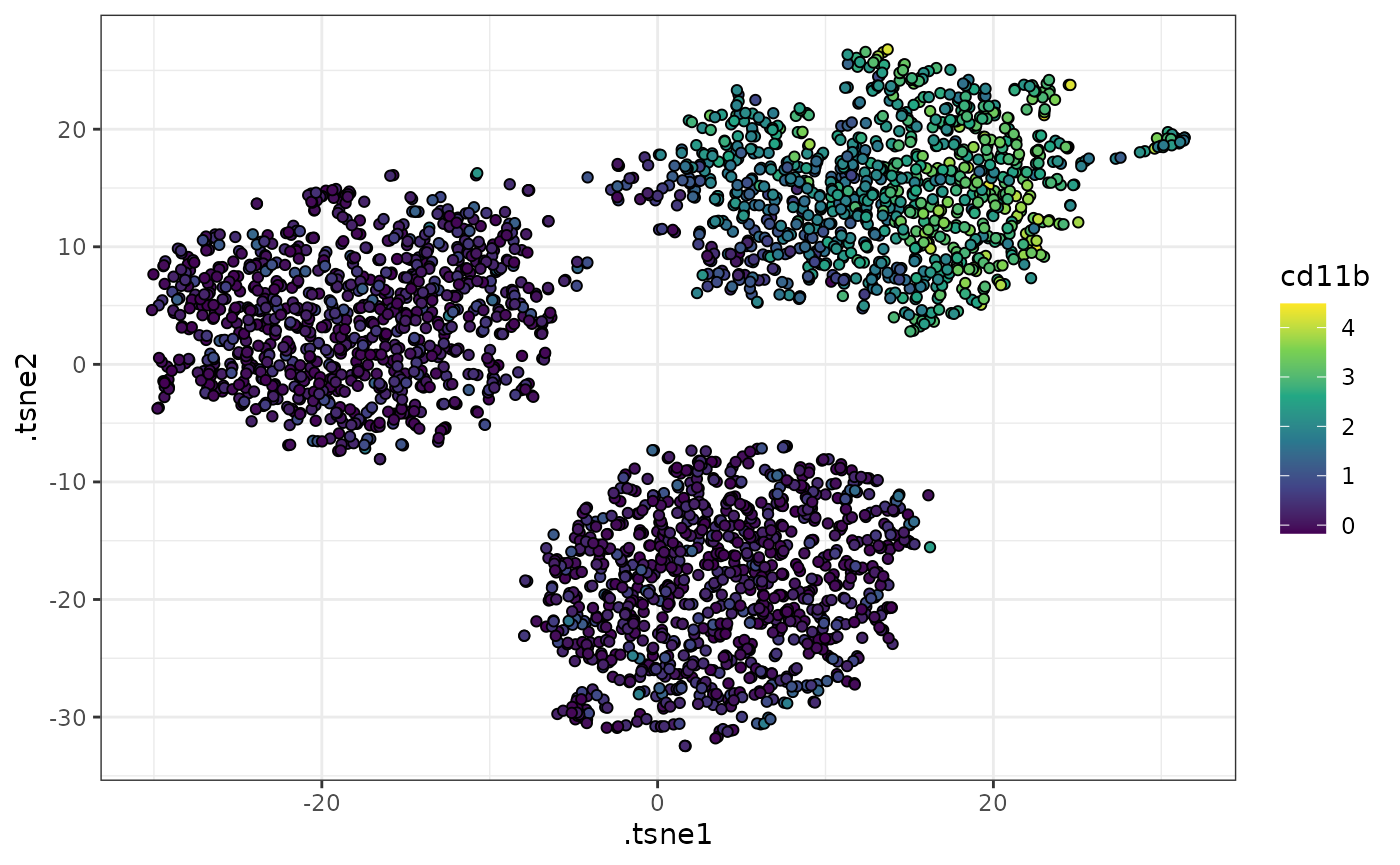
Such visualizations can be helpful in qualitatively describing the phenotypic differences between the clusters in a dataset. For example, in the example above, we can see that one of the clusters has high CD11b expression, whereas the others have lower CD11b expression.
Session info
sessionInfo()
#> R version 4.4.1 (2024-06-14)
#> Platform: x86_64-pc-linux-gnu
#> Running under: Ubuntu 22.04.4 LTS
#>
#> Matrix products: default
#> BLAS:   /usr/lib/x86_64-linux-gnu/openblas-pthread/libblas.so.3
#> LAPACK: /usr/lib/x86_64-linux-gnu/openblas-pthread/libopenblasp-r0.3.20.so;  LAPACK version 3.10.0
#>
#> locale:
#>  [1] LC_CTYPE=C.UTF-8       LC_NUMERIC=C           LC_TIME=C.UTF-8
#>  [4] LC_COLLATE=C.UTF-8     LC_MONETARY=C.UTF-8    LC_MESSAGES=C.UTF-8
#>  [7] LC_PAPER=C.UTF-8       LC_NAME=C              LC_ADDRESS=C
#> [10] LC_TELEPHONE=C         LC_MEASUREMENT=C.UTF-8 LC_IDENTIFICATION=C
#>
#> time zone: UTC
#> tzcode source: system (glibc)
#>
#> attached base packages:
#> [1] stats     graphics  grDevices utils     datasets  methods   base
#>
#> other attached packages:
#> [1] ggplot2_3.5.1  dplyr_1.1.4    tidytof_0.99.8
#>
#> loaded via a namespace (and not attached):
#>   [1] gridExtra_2.3       rlang_1.1.4         magrittr_2.0.3
#>   [4] RcppAnnoy_0.0.22    matrixStats_1.3.0   compiler_4.4.1
#>   [7] systemfonts_1.1.0   vctrs_0.6.5         stringr_1.5.1
#>  [10] pkgconfig_2.0.3     shape_1.4.6.1       fastmap_1.2.0
#>  [13] labeling_0.4.3      ggraph_2.2.1        utf8_1.2.4
#>  [16] rmarkdown_2.28      prodlim_2024.06.25  tzdb_0.4.0
#>  [19] ragg_1.3.2          purrr_1.0.2         xfun_0.47
#>  [22] glmnet_4.1-8        cachem_1.1.0        jsonlite_1.8.8
#>  [25] recipes_1.1.0       highr_0.11          tweenr_2.0.3
#>  [28] irlba_2.3.5.1       parallel_4.4.1      R6_2.5.1
#>  [31] bslib_0.8.0         stringi_1.8.4       parallelly_1.38.0
#>  [34] rpart_4.1.23        lubridate_1.9.3     jquerylib_0.1.4
#>  [37] Rcpp_1.0.13         iterators_1.0.14    knitr_1.48
#>  [40] future.apply_1.11.2 readr_2.1.5         flowCore_2.16.0
#>  [43] Matrix_1.7-0        splines_4.4.1       nnet_7.3-19
#>  [46] igraph_2.0.3        timechange_0.3.0    tidyselect_1.2.1
#>  [49] yaml_2.3.10         viridis_0.6.5       timeDate_4032.109
#>  [52] doParallel_1.0.17   codetools_0.2-20    listenv_0.9.1
#>  [55] lattice_0.22-6      tibble_3.2.1        Biobase_2.64.0
#>  [58] withr_3.0.1         evaluate_0.24.0     Rtsne_0.17
#>  [61] future_1.34.0       desc_1.4.3          survival_3.6-4
#>  [64] polyclip_1.10-7     embed_1.1.4         pillar_1.9.0
#>  [67] foreach_1.5.2       stats4_4.4.1        generics_0.1.3
#>  [70] RcppHNSW_0.6.0      S4Vectors_0.42.1    hms_1.1.3
#>  [73] munsell_0.5.1       scales_1.3.0        globals_0.16.3
#>  [76] class_7.3-22        glue_1.7.0          tools_4.4.1
#>  [79] data.table_1.15.4   gower_1.0.1         fs_1.6.4
#>  [82] graphlayouts_1.1.1  tidygraph_1.3.1     grid_4.4.1
#>  [85] yardstick_1.3.1     tidyr_1.3.1         RProtoBufLib_2.16.0
#>  [88] ipred_0.9-15        colorspace_2.1-1    ggforce_0.4.2
#>  [91] cli_3.6.3           textshaping_0.4.0   fansi_1.0.6
#>  [94] cytolib_2.16.0      viridisLite_0.4.2   lava_1.8.0
#>  [97] uwot_0.2.2          gtable_0.3.5        sass_0.4.9
#> [100] digest_0.6.37       BiocGenerics_0.50.0 ggrepel_0.9.5
#> [103] htmlwidgets_1.6.4   farver_2.1.2        memoise_2.0.1
#> [106] htmltools_0.5.8.1   pkgdown_2.1.0       lifecycle_1.0.4
#> [109] hardhat_1.4.0       MASS_7.3-60.2