GETTING STARTED with tidytof

Analyzing single-cell data can be surprisingly complicated. This is partially because single-cell data analysis is an incredibly active area of research, with new methods being published on a weekly - or even daily! - basis. Accordingly, when new tools are published, they often require researchers to learn unique, method-specific application programming interfaces (APIs) with distinct requirements for input data formatting, function syntax, and output data structure. On the other hand, analyzing single-cell data can be challenging because it often involves simultaneously asking questions at multiple levels of biological scope - the single-cell level, the cell subpopulation (i.e. cluster) level, and the whole-sample or whole-patient level - each of which has distinct data processing needs.

To address both of these challenges for high-dimensional cytometry, tidytof (“tidy” as in “tidy data”; “tof” as in “CyTOF”, a flagship high-dimensional cytometry technology) implements a concise, integrated “grammar” of single-cell data analysis capable of answering a variety of biological questions. Available as an open-source R package, tidytof provides an easy-to-use pipeline for analyzing high-dimensional cytometry data by automating many common data-processing tasks under a common “tidy data” interface. This vignette introduces you to the tidytof’s high-level API and shows quick examples of how they can be applied to high-dimensional cytometry datasets.

Prerequisites

tidytof makes heavy use of two concepts that may be unfamiliar to R beginners. The first is the pipe (|>), which you can read about here. The second is “grouping” data in a data.frame or tibble using dplyr::group_by, which you can read about here. Most tidytof users will also benefit from a relatively in-depth understanding of the dplyr package, which has a wonderful introductory vignette here:

vignette("dplyr")

Everything else should be self-explanatory for both beginner and advanced R users, though if you have zero background in running R code, you should read this chapter of R for Data Science by Hadley Wickham.

Workflow basics

Broadly speaking, tidytof’s functionality is organized to support the 3 levels of analysis inherent to single-cell data described above:

Reading, writing, preprocessing, and visualizing data at the level of individual cells
Identifying and describing cell subpopulations or clusters
Building models (for inference or prediction) at the level of patients or samples

tidytof provides functions (or “verbs”) that operate at each of these levels of analysis:

Cell-level data:
- tof_read_data() reads single-cell data from FCS or CSV files on disk into a tidy data frame called a tof_tbl. tof_tbls represent each cell as a row and each protein measurement (or other piece of information associated with a given cell) as a column.
- tof_preprocess() transforms protein expression values using a user-provided function (i.e. log-transformation, centering, scaling)
- tof_downsample() reduces the number of cells in a tof_tibble via subsampling.
- tof_reduce_dimensions() performs dimensionality reduction (across columns)
- tof_write_data writes single-cell data in a tof_tibble back to disk in the form of an FCS or CSV file.
Cluster-level data:
- tof_cluster() clusters cells using one of several algorithms commonly applied to high-dimensional cytometry data
- tof_metacluster() agglomerates clusters into a smaller number of metaclusters
- tof_analyze_abundance() performs differential abundance analysis (DAA) for clusters or metaclusters across experimental groups
- tof_analyze_expression() performs differential expression analysis (DEA) for clusters’ or metaclusters’ marker expression levels across experimental groups
- tof_extract_features() computes summary statistics (such as mean marker expression) for each cluster. Also (optionally) pivots these summary statistics into a sample-level tidy data frame in which each row represents a sample and each column represents a cluster-level summary statistic.
Sample-level data:
- tof_split_data() splits sample-level data into a training and test set for predictive modeling
- tof_create_grid() creates an elastic net hyperparameter search grid for model tuning
- tof_train_model() trains a sample-level elastic net model and saves it as a tof_model object
- tof_predict() Applies a trained tof_model to new data to predict sample-level outcomes
- tof_assess_model() calculates performance metrics for a trained tof_model

{tidytof} verb syntax

With very few exceptions, tidytof functions follow a specific, shared syntax that involves 3 types of arguments that always occur in the same order. These argument types are as follows:

For almost all tidytof functions, the first argument is a data frame (or tibble). This enables the use of the pipe (|>) for multi-step calculations, which means that your first argument for most functions will be implicit (passed from the previous function using the pipe). This also means that most tidytof functions are so-called “single-table verbs,” with the exception of tof_cluster_ddpr, which is a “two-table verb” (for details about how to use tof_cluster_ddpr, see the “clustering-and-metaclustering” vignette).
The second group of arguments are called column specifications, and they end in the suffix _col or _cols. Column specifications are unquoted column names that tell a tidytof verb which columns to compute over for a particular operation. For example, the cluster_cols argument in tof_cluster allows the user to specify which column in the input data frames should be used to perform the clustering. Regardless of which verb requires them, column specifications support tidyselect helpers and follow the same rules for tidyselection as tidyverse verbs like dplyr::select() and tidyr::pivot_longer().
Finally, the third group of arguments for each tidytof verb are called method specifications, and they’re comprised of every argument that isn’t an input data frame or a column specification. Whereas column specifications represent which columns should be used to perform an operation, method specifications represent the details of how that operation should be performed. For example, the tof_cluster_phenograph() function requires the method specification num_neighbors, which specifies how many nearest neighbors should be used to construct the PhenoGraph algorithm’s k-nearest-neighbor graph. In most cases, tidytof sets reasonable defaults for each verb’s particular method specifications, but your workflows are can also be customized by experimenting with non-default values.

The following code demonstrates how tidytof verb syntax looks in practice, with column and method specifications explicitly pointed out:

data(ddpr_data)

set.seed(777L)

ddpr_data |>
    tof_preprocess() |>
    tof_cluster(
        cluster_cols = starts_with("cd"), # column specification
        method = "phenograph", # method specification,
    ) |>
    tof_metacluster(
        cluster_col = .phenograph_cluster, # column specification
        num_metaclusters = 4, # method specification
        method = "kmeans" # method specification
    ) |>
    tof_downsample(
        group_cols = .kmeans_metacluster, # column specification
        num_cells = 200, # method specification
        method = "constant" # method specification
    ) |>
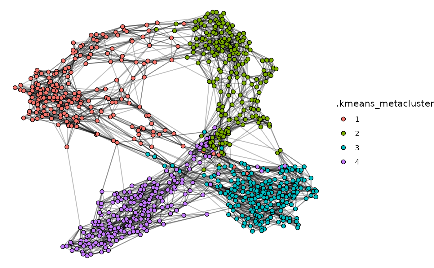
    tof_plot_cells_layout(
        knn_cols = starts_with("cd"), # column specification
        color_col = .kmeans_metacluster, # column specification
        num_neighbors = 7L, # method specification
        node_size = 2L # method specification
    )

Pipelines

tidytof verbs can be used on their own or in combination with one another using the pipe (|>) operator. For example, here is a multistep “pipeline” that takes a built-in tidytof dataset and performs the following analytical steps:

Arcsinh-transform each column of protein measurements (the default behavior of the tof_preprocess verb
Cluster our cells based on the surface markers in our panel
Downsample the dataset such that 100 random cells are picked from each cluster
Perform dimensionality reduction on the downsampled dataset using tSNE
Visualize the clusters using a low-dimensional tSNE embedding

ddpr_data |>
    # step 1
    tof_preprocess() |>
    # step 2
    tof_cluster(
        cluster_cols = starts_with("cd"),
        method = "phenograph",
        # num_metaclusters = 4L,
        seed = 2020L
    ) |>
    # step 3
    tof_downsample(
        group_cols = .phenograph_cluster,
        method = "constant",
        num_cells = 400
    ) |>
    # step 4
    tof_reduce_dimensions(method = "tsne") |>
    # step 5
    tof_plot_cells_embedding(
        embedding_cols = contains("tsne"),
        color_col = .phenograph_cluster
    ) +
    ggplot2::theme(legend.position = "none")
#> Loading required namespace: Rtsne

Other tips

tidytof was designed by a multidisciplinary team of wet-lab biologists, bioinformaticians, and physician-scientists who analyze high-dimensional cytometry and other kinds of single-cell data to solve a variety of problems. As a result, tidytof’s high-level API was designed with great care to mirror that of the tidyverse itself - that is, to be human-centered, consistent, composable, and inclusive for a wide userbase.

Practically speaking, this means a few things about using tidytof.

First, it means that tidytof was designed with a few quality-of-life features in mind. For example, you may notice that most tidytof functions begin with the prefix tof_. This is intentional, as it will allow you to use your development environment’s code-completing software to search for tidytof functions easily (even if you can’t remember a specific function name). For this reason, we recommend using tidytof within the RStudio development environment; however, many code editors have predictive text functionality that serves a similar function. In general, tidytof verbs are organized in such a way that your IDE’s code-completion tools should also allow you to search for (and compare) related functions with relative ease. (For instance, the tof_cluster_ prefix is used for all clustering functions, and the tof_downsample_ prefix is used for all downsampling functions).

Second, it means that tidytof functions should be relatively intuitive to use due to their shared logic - in other words, if you understand how to use one tidytof function, you should understand how to use most of the others. An example of shared logic across tidytof functions is the argument group_cols, which shows up in multiple verbs (tof_downsample, tof_cluster, tof_daa, tof_dea, tof_extract_features, and tof_write_data). In each case, group_cols works the same way: it accepts an unquoted vector of column names (specified manually or using tidyselection) that should be used to group cells before an operation is performed. This idea generalizes throughout tidytof: if you see an argument in one place, it will behave identically (or at least very similarly) wherever else you encounter it.

Finally, it means that tidytof is optimized first for ease-of-use, then for performance. Because humans and computers interact with data differently, there is always a trade-off between choosing a data representation that is intuitive to a human user vs. choosing a data representation optimized for computational speed and memory efficiency. When these design choices conflict with one another, our team tends to err on the side of choosing a representation that is easy-to-understand for users even at the expense of small performance costs. Ultimately, this means that tidytof may not be the optimal tool for every high-dimensional cytometry analysis, though hopefully its general framework will provide most users with some useful functionality.

Where to go next

tidytof includes multiple vignettes that cover different components of the prototypical high-dimensional cytometry data analysis pipeline. To learn the basics, we recommend visiting the vignettes in the following order to start with smalle (cell-level) operations and work your way up to larger (cluster- and sample-level) operations:

Reading and writing data
Preprocessing
Quality control
Downsampling
Dimensionality reduction
Clustering and metaclustering
Differential discovery analysis
Feature extraction
Modeling

You can also read the academic papers describing {tidytof} and/or the larger tidyomics initiative of which tidytof is a part. You can also visit the tidytof website.

Session info

sessionInfo()
#> R version 4.4.0 (2024-04-24)
#> Platform: x86_64-pc-linux-gnu
#> Running under: Ubuntu 22.04.4 LTS
#> 
#> Matrix products: default
#> BLAS:   /usr/lib/x86_64-linux-gnu/openblas-pthread/libblas.so.3 
#> LAPACK: /usr/lib/x86_64-linux-gnu/openblas-pthread/libopenblasp-r0.3.20.so;  LAPACK version 3.10.0
#> 
#> locale:
#>  [1] LC_CTYPE=C.UTF-8       LC_NUMERIC=C           LC_TIME=C.UTF-8       
#>  [4] LC_COLLATE=C.UTF-8     LC_MONETARY=C.UTF-8    LC_MESSAGES=C.UTF-8   
#>  [7] LC_PAPER=C.UTF-8       LC_NAME=C              LC_ADDRESS=C          
#> [10] LC_TELEPHONE=C         LC_MEASUREMENT=C.UTF-8 LC_IDENTIFICATION=C   
#> 
#> time zone: UTC
#> tzcode source: system (glibc)
#> 
#> attached base packages:
#> [1] stats     graphics  grDevices utils     datasets  methods   base     
#> 
#> other attached packages:
#> [1] tidytof_0.99.7
#> 
#> loaded via a namespace (and not attached):
#>   [1] gridExtra_2.3       rlang_1.1.3         magrittr_2.0.3     
#>   [4] matrixStats_1.3.0   compiler_4.4.0      systemfonts_1.0.6  
#>   [7] vctrs_0.6.5         stringr_1.5.1       pkgconfig_2.0.3    
#>  [10] shape_1.4.6.1       fastmap_1.1.1       labeling_0.4.3     
#>  [13] ggraph_2.2.1        utf8_1.2.4          rmarkdown_2.26     
#>  [16] prodlim_2023.08.28  tzdb_0.4.0          ragg_1.3.0         
#>  [19] purrr_1.0.2         xfun_0.43           glmnet_4.1-8       
#>  [22] cachem_1.0.8        jsonlite_1.8.8      recipes_1.0.10     
#>  [25] highr_0.10          tweenr_2.0.3        parallel_4.4.0     
#>  [28] R6_2.5.1            bslib_0.7.0         stringi_1.8.3      
#>  [31] parallelly_1.37.1   rpart_4.1.23        lubridate_1.9.3    
#>  [34] jquerylib_0.1.4     Rcpp_1.0.12         iterators_1.0.14   
#>  [37] knitr_1.46          future.apply_1.11.2 readr_2.1.5        
#>  [40] flowCore_2.16.0     Matrix_1.7-0        splines_4.4.0      
#>  [43] nnet_7.3-19         igraph_2.0.3        timechange_0.3.0   
#>  [46] tidyselect_1.2.1    yaml_2.3.8          viridis_0.6.5      
#>  [49] timeDate_4032.109   doParallel_1.0.17   codetools_0.2-20   
#>  [52] listenv_0.9.1       lattice_0.22-6      tibble_3.2.1       
#>  [55] Biobase_2.64.0      withr_3.0.0         Rtsne_0.17         
#>  [58] evaluate_0.23       future_1.33.2       desc_1.4.3         
#>  [61] survival_3.5-8      polyclip_1.10-6     pillar_1.9.0       
#>  [64] foreach_1.5.2       stats4_4.4.0        generics_0.1.3     
#>  [67] RcppHNSW_0.6.0      S4Vectors_0.42.0    hms_1.1.3          
#>  [70] ggplot2_3.5.1       munsell_0.5.1       scales_1.3.0       
#>  [73] globals_0.16.3      class_7.3-22        glue_1.7.0         
#>  [76] tools_4.4.0         data.table_1.15.4   gower_1.0.1        
#>  [79] fs_1.6.4            graphlayouts_1.1.1  tidygraph_1.3.1    
#>  [82] grid_4.4.0          yardstick_1.3.1     tidyr_1.3.1        
#>  [85] RProtoBufLib_2.16.0 ipred_0.9-14        colorspace_2.1-0   
#>  [88] ggforce_0.4.2       cli_3.6.2           textshaping_0.3.7  
#>  [91] fansi_1.0.6         cytolib_2.16.0      viridisLite_0.4.2  
#>  [94] lava_1.8.0          dplyr_1.1.4         gtable_0.3.5       
#>  [97] sass_0.4.9          digest_0.6.35       BiocGenerics_0.50.0
#> [100] ggrepel_0.9.5       htmlwidgets_1.6.4   farver_2.1.1       
#> [103] memoise_2.0.1       htmltools_0.5.8.1   pkgdown_2.0.9      
#> [106] lifecycle_1.0.4     hardhat_1.3.1       MASS_7.3-60.2

Timothy Keyes